ONE SAMPLE T-TEST USING R CONSOLE 

Q. 10 pieces of sarees were selected and number of defects were calculated as: 4, 4,0,3,3,2,3,5,8,6,6

test weather average number of defects on such a cloth is less than 5. 

Sol.

Step I:  we want to test a null hypothesis

                  H0:   mu = 5

against an alternating hypothesis

                  H1:   mu < 5

Step II:  Test statistic
t = x_bar - mu_not/(s/sqrt(n))  ~ t_(n-1)

where s^2=(1/n-1) summation(1 to n)(x_i - x_bar)^2 ~ t_(n-1)

and x_bar = (1/n) summation(1 to n)x_i 

Command used: 

> defect=c(4,0,3,3,2,3,5,8,6,6)
> t.test(defect,alt="less",mu=5)

        One Sample t-test

data:  defect
t = -1.3693, df = 9, p-value = 0.102
alternative hypothesis: true mean is less than 5
95 percent confidence interval:
     -Inf 5.338716
sample estimates:
mean of x
        4

Conclusion:  Since the p-values is greater than 0.05 so we accept the null hypothesis.

How to fit a multiple linear regression equation in R.


> y=scan()    [enter y values]
1: 10
2: 20
3: 50
4: 70
5: 90
6: 100
7: 130
8: 150
9: 155
10: 160
11: 155
12
Read 11 items
> x1=scan()    [enter x1values]
1: 50
2: 50
3: 50
4: 51
5: 52
6: 53
7: 54
8: 55
9: 55
10: 56
11: 58
12:
Read 11 items
> x2=scan()       [enter x2 values]
1: 1
2: 1.2
3: 1.5
4: 2
5: 2.5
6: 3
7: 3.3
8: 4
9: 6
10: 6.5
11: 7.5
12:
Read 11 items
> df=data.frame(y,x1,x2)    [represent data in tabular form]
> df
     y x1  x2
1   10 50 1.0
2   20 50 1.2
3   50 50 1.5
4   70 51 2.0
5   90 52 2.5
6  100 53 3.0
7  130 54 3.3
8  150 55 4.0
9  155 55 6.0
10 160 56 6.5
11 155 58 7.5
> cor(df)                                                     [get rank correlation coefficient of y on x1 and x2]
           y        x1        x2
y  1.0000000 0.9350985 0.8942423
x1 0.9350985 1.0000000 0.9617563
x2 0.8942423 0.9617563 1.0000000
> model=lm(y~x1+x2)                            [to fit regression equation of y on x1 and x2]
> model

Call:                                                         [output result]
lm(formula = y ~ x1 + x2)

Coefficients:
(Intercept)           x1           x2
   -976.197       20.365       -1.682

How to find covariance, correlation coefficient, spearman's coefficient, regression line, estimated value, residual value for data stored in x, y.

> x=scan()    [enter x data]
1: 56
2: 47
3: 33
4: 39
5: 42
6: 38
7: 46
8: 47
9: 38
10: 32
11:
Read 10 items
> y=scan()         []enter y data]
1: 56
2: 83
3: 49
4: 52
5: 65
6: 52
7: 56
8: 48
9: 59
10: 70
11:
Read 10 items

> cov(x,y)        [to get covariance of x, y]
[1] 4.444444

> cor(x,y)           [to get correlation coefficient]
[1] 0.05560642
> cor(x,y,method="spearman")   [to get spearman's coefficient]
[1] -0.003067485
> model=lm(y~x)      [to fit regression equation]
> model

Call:                                         [result output]
lm(formula = y ~ x)

Coefficients:
(Intercept)            x 
   55.54260      0.08271 


> plot(x,y,col="red")            [plot x, y points]    
> abline(model,h=0,v=0,col="blue")  [plot regression line]
> model$fitted[6]                     [to get fitted value]
       6
58.68569
> model$residuals[6]                [to get residual value]
        6
-6.685691

Measure of central tendency and measure of dispersion using R console:

> age1=scan()      [enter data by variable age1]
1: 20
2: 24
3: 19
4: 24
5: 18
6: 19
7: 24
8: 22
9: 23
10: 19
11: 19
12: 24
13: 2
14: 21
15: 22
16: 23
17: 24
18: 21
19: 25
20: 23
21:
Read 20 items
> mean(age1)      [to find mean]
[1] 20.8
> median(age1)    [to find median]
[1] 22
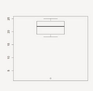
> summary(age1)    [to find min., 1st, 3rd quartile, mean, median, max. at a time]
   Min. 1st Qu.  Median    Mean 3rd Qu.    Max.
    2.0    19.0    22.0    20.8    24.0    25.0
> quantile(age1)                                        [to find n percentile]
  0%  25%  50%  75% 100%
   2   19   22   24   25
> IQR(age1)   [to find inter quartile range]
[1] 5
> var(age1)     [to find variance]
[1] 24.27368
> sd(age1)      [to find S.D. ]
[1] 4.926833
> boxplot(age1, lables=T)    [to draw boxplot of data]

How to draw a frequency polygon using R-console:

> age=scan()
1: 20
2: 24
3: 19
4: 24
5: 18
6: 19
7: 24
8: 22
9: 23
10: 19
11: 19
12: 24
13: 2
14: 21
15: 22
16: 23
17: 24
18: 21
19: 25
20: 23
21:
Read 20 items
> freq=table(age1)
> cumfreq=cumsum(freq)                          
> plot(freq, type="o", col=color)
 plot(cumfreq, type="o", col=color)

How to divide data in different class interval to get frequency, cumulative frequency of a particular class interval:


> age=scan()
1: 20
2: 24
3: 19
4: 24
5: 18
6: 19
7: 24
8: 22
9: 23
10: 19
11: 19
12: 24
13: 2
14: 21
15: 22
16: 23
17: 24
18: 21
19: 25
20: 23
21:
Read 20 items
> range(age)
[1]  2 25
> interval=seq(1,27,2)          [taking less values for start and greater value for end to the given range]
> class=cut(age1,interval,right=F)    [to get class interval]
> freq=table(class)                             [to get frequency of individual class interval]
> freq
class
  [1,3)   [3,5)   [5,7)   [7,9)  [9,11) [11,13) [13,15) [15,17) [17,19) [19,21)
      1       0       0       0       0       0       0       0       1       5
[21,23) [23,25) [25,27)
      4       8       1


> cumfreq=cumsum(freq)
> cumfreq
  [1,3)   [3,5)   [5,7)   [7,9)  [9,11) [11,13) [13,15) [15,17) [17,19) [19,21)
      1       1       1       1       1       1       1       1       2       7
[21,23) [23,25) [25,27)
     11      19      20

How to draw bar plot and pie chart of a frequency distribution from a given data:
Example:
> age=scan()   [enter age of some woman by variable age]
1: 20
2: 24
3: 19
4: 24
5: 18
6: 19
7: 24
8: 22
9: 23
10: 19
11: 19
12: 24
13: 2
14: 21
15: 22
16: 23
17: 24
18: 21
19: 25
20: 23
                            [enter two times to stop entering process]
Read 20 items
> freq=table(age)
> cumfreq=cumsum(freq)
> cbind(freq, cumfreq)
   freq cumfreq
2     1       1
18    1       2
19    4       6
20    1       7
21    2       9
22    2      11
23    3      14
24    5      19
25    1      20
> color=c("red", "green", "blue")     [to define color]
> barplot(freq,col=color)                  [to draw bar plot with defined colors]
> pie(freq, col=color)                        [to draw pie chart with defined colors]

How to find frequency, cummulative frequency, percent  and cumulative percent using R-console:

Ex.
> var1=c(23,26,24,25,26,23,26,25,25,27,24,24,22,22)
> freq=table(var1)
> cumfreq=cumsum(freq)
> pct=freq*100/length(var1)
> cumpct=cumsum(pct)
> cbind(freq, cumfreq,pct,cumpct)
   freq            cumfreq               pct                cumpct
22                    2       2             14.285714       14.28571
23                    2       4             14.285714       28.57143
24                    3       7             21.428571       50.00000
25                    3      10            21.428571       71.42857
26                    3      13            21.428571       92.85714
27                    1      14            7.142857         100.00000
> 

How to calculate frequency and cumulative frequency using R-console:

syntex for cumulative frequency:
var1=c()                                [to enter data by var1]
freq=table(var1)                  [to find frequency from var1]
cumfreq=cumsum(freq)      [to find cumulative frequency from frequency]
cbind(freq,cumfreq)             [to represent frequency, cumulative frequency in a table]
  
Ex. 
> var1=c(23,26,24,25,26,23,26,25,25,27,24,24,22,22)
> freq=table(var1)
> cumfreq=cumsum(freq)
> cbind(freq,cumfreq)
   freq cumfreq
22    2       2
23    2       4
24    3       7
25    3      10
26    3      13
27    1      14


 

Basic mathematical operations in R-console

Quotient:

syntex  divident/divisor=quotient
Ex. > 7/2
[1] 3.5

Integral quotient:
syntex   divident%/%divisor=integral quotient
Ex.
> 7%/%2
[1] 3 

Remainder:
syntex  divident%%divisor=remainder
Ex.
> 10%%3
[1] 1

Length of a string

syntex  length('var')

Ex.
> x=seq(1,9,0.5)
> x
 [1] 1.0 1.5 2.0 2.5 3.0 3.5 4.0 4.5 5.0 5.5 6.0 6.5 7.0 7.5 8.0 8.5 9.0
> length(x)
[1] 17

Repeat n times a set of data
syntex  new _var=rep(existing_var, c(n)) 

Ex.
> y=rep(x,c(5))
> y
 [1] 1.0 1.5 2.0 2.5 3.0 3.5 4.0 4.5 5.0 5.5 6.0 6.5 7.0 7.5 8.0 8.5 9.0 1.0 1.5
[20] 2.0 2.5 3.0 3.5 4.0 4.5 5.0 5.5 6.0 6.5 7.0 7.5 8.0 8.5 9.0 1.0 1.5 2.0 2.5
[39] 3.0 3.5 4.0 4.5 5.0 5.5 6.0 6.5 7.0 7.5 8.0 8.5 9.0 1.0 1.5 2.0 2.5 3.0 3.5
[58] 4.0 4.5 5.0 5.5 6.0 6.5 7.0 7.5 8.0 8.5 9.0 1.0 1.5 2.0 2.5 3.0 3.5 4.0 4.5
[77] 5.0 5.5 6.0 6.5 7.0 7.5 8.0 8.5 9.0
> length(y)
[1] 85

Continue....R-commands

3. To enter data in a range[START-END]
Example
> x=c(1:80)      [enter data from 1 to 80 associated with a variable x]
> x                    [to read entered data]
 [1]  1  2  3  4  5  6  7  8  9 10 11 12 13 14 15 16 17 18 19 20 21 22 23 24 25
[26] 26 27 28 29 30 31 32 33 34 35 36 37 38 39 40 41 42 43 44 45 46 47 48 49 50
[51] 51 52 53 54 55 56 57 58 59 60 61 62 63 64 65 66 67 68 69 70 71 72 73 74 75
[76] 76 77 78 79 80

Ex.  enter data from 1-10 and than 2
> x=c(1:10,2)
> x
 [1]  1  2  3  4  5  6  7  8  9 10  2








 4. To add/remove/change entered data x
> data.entry(x)
> x
 [1]  1  2  3  4  5  6  7  8  9 10 NA   [we remove 2 from x]
> de(x)                                             [command work same as data.entry]
>x
 [1]  1  2  3  4  5  6  7  8  9 10 NA


5. To enter data in a sequence with specified interval:

syntex        a= seq(start, end, interval)

Ex. a=seq(1, 100, 0.5)

R-Console basic commands

1. To enter data in vertical form

x = scan()

for example
> x=scan()
1: 1
2: 2
3: 3
4: 4
!
!
!
and so on

2. To enter data in horizontal form

>y=c(1,3,5,7.......and so on)